Carbon 1s for Organic Compounds

The seminal work of Graham Beamson and Dave Briggs in their "High Resolution XPS of Organic Polymers – The Scienta ESCA300 Database" has been utilized since 1992 as an invaluable resource for the XPS analysis of polymers and organic materials.  A summary of carbon 1s binding energies for organic functional groups from this work are presented here. The original work calibrates the binding energy scale to 285.0 eV for aliphatic carbon C 1s. The values presented here are now calibrated to 284.8 eV for aliphatic carbon, in line with recent results [2].  

Figure 1. Summary of the mean, maximum, and minimum carbon 1s binding energies for different organic functionalities according to the work of Beamson and Briggs [1].  Binding energy calibration presented here have been adjusted to the main aliphatic C 1s peak at 284.8 eV.

Table 1. Summary of the mean, maximum, and minimum carbon 1s binding energies for different organic functionalities according to the work of Beamson and Briggs [1].  Binding energy calibration presented here have been adjusted to the main aliphatic C 1s peak at 284.8 eV.

Table 2. Summary of beta shift effects from Beamson and Briggs (Appendix 2) [1].

The effects of various functional groups on beta carbon binding energies can be significant (Table 2).  Note that, in this context, the alpha carbon is the carbon directly attached to the functional group, and the beta carbon is attached to the alpha carbon. These effects have been included in the refinement of the binding energy value for the aliphatic carbon component in adventitious carbon [2]. 

References:
[1] G. Beamson, D. Briggs, High Resolution XPS of Organic Polymers - The Scienta ESCA300 Database, Wiley Interscience, 1992, Appendices 1 and 2.
[2] L.H. Grey, H.-Y. Nie, M.C. Biesinger, Appl. Surf. Sci. 653 (2024) 159319.

Calculating Oxygen Content from Adventitious Carbon 1s Spectra

Adventitious carbon (AdC) is commonly detected in X-ray photoelectron spectroscopy (XPS) analyses of most samples. While AdC can be beneficial in some cases, such as for charge correction purposes during the analysis of insulators, its associated C–O functionalities can complicate the interpretation of O 1s spectra. Accurately accounting for AdC’s contribution within the O 1s spectrum is essential but challenging due to significant spectral overlap and poorly resolved components in the high-resolution O 1s spectrum.

Rather than assigning multiple components without clear physical meaning—potentially leading to misinterpretations—incorporating stoichiometry offers a more reliable approach to improving data accuracy. However, applying stoichiometry can be tedious and challenging, particularly for novice users.

A recently published article [1] describes an approximation to enhance oxygen spectra interpretation by estimating oxygen linked to AdC. This publication provides background information, key assumptions, and an easy-to-use Excel calculator to assist XPS researchers in analyzing their own O 1s spectra.

This approach is particularly useful for accurately quantifying survey spectra when AdC influence must be minimized and for modelling high-binding-energy components in the oxygen 1s spectrum. The latter example is important to many transition metal oxides which have overlapping hydroxide and/or defect oxide components in the same binding energy window. Detailed examples of these applications are presented and discussed in reference [1]. These types of calculations were originally introduced in [2].

This Excel based calculator (also available at supplementary material in [1]) takes information from the survey and high resolution carbon 1s spectra and determines the amount of oxygen that is present from adventitious carbon species. This amount can then be deducted from the overall oxygen concentration.
(Note: you must download the file to Excel to use it - it is locked in Google Docs).

References:

[1] J.D. Henderson, B.P. Payne, N.S. McIntyre, M.C. Biesinger, Surf. Interface Anal. 57 (2025) 214-220.
[2] B.P. Payne, M.C. Biesinger, N.S. McIntyre, J. Electron Spectrosc. Relat. Phenom. 184 (2011) 29-37.

What is Adventitious Carbon?

A thin layer of carbonaceous material is usually found on the surface of most air exposed samples, this layer is generally known as adventitious carbon. Even small exposures to atmosphere can produce these films. Adventitious carbon is generally comprised of a variety of (relatively short chain [1]) hydrocarbons species with small amounts of both singly and doubly bound oxygen functionality. The source of this carbon has been debated over the years. It does not appear to be graphitic in nature and in most modern high vacuum systems vacuum oils are not readily present (as they have been in the past) [1,2,3,4]. There may be some evidence that CO or CO2 species may play a role in the gradual appearance of carbon on pristine surfaces within the vacuum of the XPS chamber [3].

It’s presence on insulating surfaces provides for a convenient charge reference by setting the main line of the C 1s spectrum to 284.8 eV (although values ranging from 285.0 eV to 284.5 eV have been used in some cases, remember to check for this value when looking for binding energy references in the literature). The error in this value (284.8 eV) is, for most systems, on the order of +/-0.2 eV to 0.3 eV.  An in-depth look at the effectiveness of using AdC for charge correction purposes, including standardized fitting procedures, is presented in [5].

  

Work by Grey et al. [6] has explored the nature of adventitious carbon by XPS and time-of-flight secondary ion mass spectrometry (ToF-SIMS).  XPS D-parameter and ToF-SIMS analyses confirms that AdC is not graphitic in nature. An average C 1s spectrum for AdC (Figure 1, Table 1) was derived and shows that, on average, ~ 25 % of the carbon species in AdC is directly associated with oxygen functionality.  Similarly, ToF-SIMS analyses show that AdC is comprised of mainly short chain hydrocarbons with some oxygen functionality.

An advanced method for curve-fitting of the C 1s envelope for AdC (Table 2) was developed that included the effects of beta carbons (in this context, the alpha carbon is the carbon directly attached to the oxygen, and the beta carbon is attached to the alpha carbon) and were informed by the configurations of possible volatile organic compounds (VOC) that are the source of most AdC [6]. Using this method in combination with the dataset from [5], the average C–C/C–H AdC aliphatic peak position was shown to be 284.81 eV (+/- 0.25 eV) via verification with a secondary internal reference.

Figure 1. Average of 80 adventitious carbon C 1s XPS spectra.

Table 1. Average adventitious carbon C 1s fitting parameters from an average of 80 AdC spectra.

Table 2. Curve-fitting parameters for AdC C 1s including shifted beta peaks (*) (peaks E, F and G). Areas for peaks A, B, C, and D should be left unconstrained. # If peak-shape for peak D is well-defined the FWHM constraint can be removed.

References:

[1] T.L. Barr, S. Seal, J. Vac. Sci. Technol. A 13(3) (1995) 1239.

[2] P. Swift, Surf. Interface Anal. 4 (1982) 47.
[3] D.J. Miller, M.C. Biesinger, N.S. McIntyre, Surf. Interface Anal. 33 (2002) 299.
[4] H. Piao, N.S. McIntyre, Surf. Interface Anal. 33 (2002) 591.

[5] M.C. Biesinger, Appl. Surf. Sci, 597 (2022) 153681.

[6] L.H. Grey, H.-Y. Nie, M.C. Biesinger, Appl. Surf. Sci. 653 (2024) 159319.

Using Adventitious Carbon for Charge Correcting

The C 1s spectrum for adventitious carbon can be fit as follows.  A single peak, ascribed to alkyl type carbon (C-C, C-H), is fit to the main peak of the C 1s spectrum.  A second peak is added that is constrained to be 1.5 eV above the main peak, of equal FWHM to the main peak (C-C, C-H). This higher binding energy peak is ascribed to alcohol and/or ester functionality (C-OH, C-O-C). Further high binding energy components can be added if required. For example: C=O at approximately 3 eV above the main peak and O-C=O at 3.8 to 4.3 eV above the main peak. One or both of these peaks may also have to be constrained to the FWHM of the main peak if they are poorly resolved.  Reference [1] and the table below outline standard starting fitting parameters for adventitious carbon. 

Adventitious carbon C 1s curve-fitting parameters [1].

Spectra from insulating samples can then be charge corrected by shifting all peaks to the adventitious C 1s spectral component (C-C, C-H) binding energy set to 284.8 eV. There is certainly error associated with this assignment. Swift [2] lists a number of studies showing errors ranging from ±0.1eV to ±0.4 eV.  “Newer” studies (late 1970's) range from ±0.1 to ±0.3 eV. “Older” studies (late 1960's to early 1970's) were in the ±0.4eV range - however, reproducibility and resolution of the spectrometers of the time may have played a role.  Barr's [3] work from 1995 states that error in using adventitious carbon is ±0.2 eV.  Our work [4] in 2002 also suggests error in the ±0.2eV to  ±0.3eV range.  Experience with numerous conducting samples (1995 to present) and a routinely calibrated instrument have shown that the C 1s signal generally ranges from 284.7 eV to as high as 285.2 eV [5].  Reference [1] presents a detailed assessment of the analysis of insulating samples from a multi-user facility from over a 5-year period that showed an adventitious C 1s (C-C, C-H) binding of 284.91 eV ±0.25eV.  A similar study confirming the utility of the adventitious carbon technique with a similar multi-user facility analysis has been published by Morgan [6].

For organic systems, especially polymers, it is convenient to charge correct to the C-C, C-H signal set to 285.0 eV. This makes for easier comparison to the polymer handbook [7] which uses this number for charge correction.

References:
[1] M.C. Biesinger, Appl. Surf. Sci, 597 (2022) 153681.

[2] T.L. Barr, S. Seal, J. Vac. Sci. Technol. A 13(3) (1995) 1239.
[3] P. Swift, Surf. Interface Anal. 4 (1982) 47.
[4] D.J. Miller, M.C. Biesinger, N.S. McIntyre, Surf. Interface Anal. 33 (2002) 299.
[5] M.C. Biesinger, unpublished results

[6] D.J. Morgan, Surf. Interface Anal. 57 (2025) 28.
[7] G. Beamson, D. Briggs, High Resolution XPS of Organic Polymers - The Scienta ESCA300 Database Wiley Interscience, 1992.

Graphitic/Graphene/Carbon Nanotube C 1s Curve-Fitting

Materials of a graphitic nature (e.g., graphite, graphene, carbon nanotubes etc.) will have a C 1s main peak, attributed to C=C, which can be used as a charge reference set to 284.5 eV. An average of values for graphite from 21 references from the NIST database [1] is 284.46 eV with a standard deviation of 0.14 eV. Note that the well characterized value of 284.5 eV for graphitic carbon is also a strong indicator that this value is not appropriate as a value to use for AdC charge referencing. While these types of samples are generally conductive and if they can be mounted in a manor (in electrical contact with the sample stage) to take advantage of this one should do so. However, many of these types of samples come as a small volume of powders or flakes which are very difficult to mount. Usually, we mount these on a double-sided adhesive which works well but electrically isolates the sample. Oxidation of these types of samples (e.g., graphene oxide) or their functionalization (e.g., functionalized CNTs) can result in them behaving less conductively or as a mixed conductive/insulating material.  Samples where these materials are mixed with other conducting or insulating compounds can also result in a mixed conductive/insulating sample. For most of these types of samples we now electrically isolate the sample and charge reference to C 1s at 284.5 eV for the graphitic (C=C) peak.[2]

Table 1 from [2] presents general fitting parameters for graphitic, graphene and carbon nanotube type materials. These starting fitting parameters include the main peak asymmetry (defined using an asymmetric Lorentzian (LA) line shape) and π to π* shake-up satellite from a pure graphite standard sample. These fitting parameters are similar to the approach taken by Morgan (Fig. 5, Table 2) [3],  Moeini et al. (Table 1) [4],  and Gengenbach et al.[5]  It is always best to run your own standard (pure graphite, graphene, CNT etc.) to get fitting parameters appropriate for your sample type, instrument and conditions used. Slight differences in the main peak asymmetry and differing shake-up satellite position, shape and intensities are possible for differing classes of graphitic materials. See for example from Morgan[3] where HOPG and nano-onion C 1s spectra show peak-shape differences, likely due to hydrogenation of the sample. However, with this caveat stated, the parameters used based on a graphite standard have worked very well for variety of samples (134) analyzed in the five-year data survey from [2]. Figure 1(A) presents the standard graphite spectrum used to obtain the parameters presented in Table 1. The spectra from Figure 1(B, C and D) show the use of these fitting parameters from Table 1 to effectively model a variety of graphitic component containing materials. 

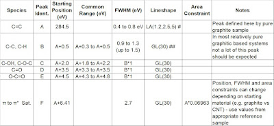
Table 1. General fitting parameters for graphitic/graphene/carbon nanotube type materials. #Line-shape details for CasaXPS. Define asymmetric peak-shape in other software using pure graphite/graphene or CNT sample related your specimens. ##Gaussian/Lorentzian product formula, GL(30) is 30% Lorentzian 70% Gaussian.[2]

Figure 1.  Examples of curve-fitting of graphitic type systems using the parameters from Table 1.  A) pure graphite, B) carbon nanotube-based material modified in caustic solution, C) oxidized graphene and D) acid modified graphene and organic compound mixture.[2]

References:
[1] C.D. Wagner, A.V. Naumkin, A. Kraut-Vass, J.W. Allison, C.J. Powell, J.R.Jr. Rumble, NIST Standard Reference Database 20, Version 3.4 (web version) (http:/srdata.nist.gov/xps/) 2003.
[2] M.C. Biesinger, Appl. Surf. Sci. 597 (2022) 153681.
[3] D.J. Morgan, J. Carbon. Res. 7 (2021) 51.
[4] B. Moeini, M.R. Linford, N. Fairley, A. Barlow, P. Cumpson, D. Morgan, V. Fernandez, J. Baltrusaitis. Surf. Interface Anal. 54 (2022) 67.
[5] T.R. Gengenbach, G.H. Major, M.R. Linford, C.D. Easton, J. Vac. Sci. Technol. A, 39 (2021) 013204.

Polyethylene Surfaces

The C 1s spectrum of polyethylene shows vibrational structure[1] that leads to an asymmetric peak-shape.  If this vibrational structure is not accounted for it can lead to an erroneous assignment of C-OH, C-O-C or an overestimate of contamination/oxidation species[2]. A fitting of a series of polyethylene standards (Figure 1) as well as a fitting of a C18 alkane (Figure 2) on a clean silicon wafer gave consistent peak-shape results and were fit with an asymmetric peak-shape defined in CasaXPS as LA(4.2,9,4) and with peak widths of 0.64-0.65 eV (at 10 eV pass energy) and 0.67-0.68 eV (at 20 eV pass energy). Peak fitting parameters for PE surfaces with small amounts of oxidation and/or contamination are presented in Table 1 and an example is shown in Figure 3. 

Table 1. Contaminated/oxidized polyethylene surface C 1s fitting parameters.

Figure 1. C 1s spectrum of a standard polyethylene sample (20 eV pass energy).

Figure 2. C 1s spectrum of C18 alkane (10 eV pass energy).

Figure 3. C 1s spectrum of a contaminated/oxidized PE surface using the fitting parameters from Table 1.

A similar analysis of polypropylene (Figure 4) gave a peak that can be fit with an asymmetric peak-shape defined in CasaXPS as LA(5.5,9,4) and with peak-widths of 0.82 eV for a 10 eV pass energy and 0.83 eV for a 20 eV pass energy.

Figure 4. C 1s spectrum of a standard polypropylene sample (20 eV pass energy).

References:
[1] G. Beamson, D. Briggs, High Resolution XPS of Organic Polymers - The Scienta ESCA300 Database Wiley Interscience, 1992.
[2] M.J. Walzak, pers. comm. 2015.

C 1s - Carbonates

The C 1s binding energy average for carbonate ((CO₃)^2-) is 289.3 +/- 0.6 eV (average of 18 carbonates, + 4.5 eV above adventitious carbon at 284.8 eV). Calcium carbonate is at 289.5 eV +/-0.1 eV or + 4.7 eV above adventitious carbon). Note that silver carbonate has a much lower binding energy at ~288.5 eV.

Graphite

Graphite and graphitic-like compounds (including carbon nanotubes) have an asymmetric C 1s peak-shape (as they are conductive) centered at 284.5 eV. Also present will be structure related to the pi to pi* transition (shake-up) at around 290.9 eV. Example shown below, click here for a CasaXPS ready file.

Polymer Databases

Some good polymer databases:

[1] G. Beamson, D. Briggs, High Resolution XPS of Organic Polymers - The Scienta ESCA300 Database, Wiley Interscience, 1992
(Note: An excellent resource, every XPS lab should have a copy!)

[2] Kratos Polymer Handbook http://www.kratos.com/EApps/polybook2a.pdf

[3] B. Vincent Crist, Handbook of Monochromatic XPS Spectra, Polymers and Polymers Damaged by X-rays, Wiley, 2000